In this post, we’ll be taking a closer look at the kernelized Stein discrepancy that provides the real utility underlying Stein variational gradient descent. Recall that the optimal perturbation direction was revealed to be, \begin{align} \phi^\star\left(y\right) = \mathbb{E}_{x\sim q}\left[k\left(x, y\right)\nabla_x\log p(x)+\nabla_x k\left(x, y\right)\right]. \end{align} This, in turn, suggests an update equation of the form, \begin{align} x_{i+1} = x_{i} + \epsilon \cdot \phi^\star\left(x_{i}\right), \end{align} where $x_i \sim q$.

The difficulty so far is that computing the theoretical expectation under $q$ of the violation of Stein’s identity for $p$ is intractable. However, we can still approximate the expectation by generating samples from $q$ and evaluating the empirical violation of Stein’s identity. In particular, consider a set a random variables that are observed from $q$, denoted $\left\{x^{(j)}\right\}_{j=1}^{n}$; the empirical optimal perturbation is simply, \begin{align} \hat{\phi}\left(y\right) = \frac{1}{n} \sum_{j=1}^{n} k\left(x^{(j)}, y\right)\nabla_x\log p(x^{(j)})+\nabla_x k\left(x^{(j)}, y\right). \end{align} The analogous update equation for transforming the random variables to more closely approximate $p$ in terms of the KL-divergence is therefore going to be \begin{align} x^{(j)}_{i+1} = x^{(j)}_{i} + \epsilon \cdot \hat{\phi}\left(x^{(j)}_{i}\right) \end{align}

The Kernel Function

It is worth paying some attention to the kernel function $k(\cdot, \cdot)$ which has, until now, been somewhat glossed over. The most commonly used kernel (and, in fact, the kernel that is used in the original paper on Stein variational gradient descent) is the squared exponential (also called the radial basis function or Gaussian kernel). The squared exponential kernel is defined to be, \begin{align} k\left(x, y\right) = \exp\left(-\frac{1}{2h}\left|\left|x-y\right|\right|_2^2\right), \end{align} where $h > 0$ is the bandwidth of the kernel. The bandwidth controls the strength of the repulsive force between $x$ and $y$: The larger the bandwidth, the greater the repulsive force. Differentiating the squared exponential kernel with respect to $x$ gives \begin{align} \nabla_x k\left(x, y\right) = -\frac{1}{h} k\left(x, y\right) \left(x-y\right)’ \end{align}

We can implement the squared exponential kernel in Python as follows.

import numpy as np
from scipy.spatial.distance import cdist


class SquaredExponentialKernel(object):
    """Squared Exponential Kernel Class"""
    def __init__(self, n_params, bandwidth=None):
        """Initialize parameters of the squared exponential kernel object."""
        self.n_params = n_params
        self.bandwidth = bandwidth

    def kernel_and_grad(self, theta):
        """Computes both the kernel matrix for the given input as well as the
        gradient of the kernel with respect to the first input, averaged over
        inputs.
        """
        # Number of particles used to sample from the distribution.
        n_particles = theta.shape[0]
        # Compute the pairwise squared Euclidean distances between all of the
        # particles.
        sq_dists = cdist(theta, theta, metric="sqeuclidean")

        # Compute the kernel matrix.
        if self.bandwidth:
            h = self.bandwidth
        else:
            h = np.median(cdist) / np.log(n_particles = 1)

        K = np.exp(-0.5 / self.bandwidth * sq_dists)
        # Compute the average of the gradient of the kernel with respect to
        # each of the particles.
        dK = np.zeros((n_particles, self.n_params))
        for i in range(n_particles):
            dK[i] = 1.0 / self.bandwidth * K[i, :].dot(theta[i] - theta)

        return K, dK

Bayesian Linear Regression

In this example, we will consider the problem of estimating a linear model where priors have been placed over the linear coefficients with a noise variance that is assumed to be known. This corresponds to the usual instance of Bayesian linear regression where we assume a prior of $\boldsymbol{\beta}\sim \mathcal{N}\left(\mathbf{0}, \sigma^2\sigma^2_{\beta}\mathbf{I}\right)$, where $\sigma_{\beta}^2$ is a Bayesian linear regression hyperparameter. The corresponding likelihood function for the model is, \begin{align} p\left(\mathbf{y}\vert \mathbf{X}, \boldsymbol{\beta}\right) = \mathcal{N}\left(\mathbf{X}\boldsymbol{\beta}, \sigma^2\right). \end{align} It is easy to verify that the unnormalized log-posterior distribution for Bayesian linear regression is, \begin{align} \log p\left(\boldsymbol{\beta}\vert \mathbf{X}, \mathbf{y}\right) =& -\frac{n}{2}\log \sigma^2 - \frac{1}{2\sigma^2} \left(\mathbf{y} - \mathbf{X}\boldsymbol{\beta}\right)’\left(\mathbf{y} - \mathbf{X}\boldsymbol{\beta}\right) \\
& - \frac{k}{2}\log \sigma^2-\frac{1}{2\sigma^2} \frac{\boldsymbol{\beta}’\boldsymbol{\beta}}{\sigma_{\beta}^2}. \end{align} The gradient with respect to $\boldsymbol{\beta}$ is simply, \begin{align} \nabla_{\boldsymbol{\beta}} \log p = \frac{1}{\sigma^2} \left(\mathbf{y} - \mathbf{X}\boldsymbol{\beta}\right)’\mathbf{X} - \frac{1}{\sigma^2_{\beta}\sigma^2} \boldsymbol{\beta} \end{align}

As we continue this example, we’ll assume a noise variance and prior variance over the linear coefficients of unity; that is, $\sigma^2_{\beta} = \sigma^2 = 1$. Before we can proceed with estimating the coefficients via Stein variational gradient descent, however, we need a class to support this kind of posterior sampling. One implementation of Stein variational gradient descent as a class in Python can be achieved as follows:

import numpy as np


class SteinSampler(object):
    """Stein Sampler Class"""
    def __init__(self, grad_log_p, kernel, verbose=True):
        """Initialize parameters of the Stein sampler."""
        self.grad_log_p = grad_log_p
        self.kernel = kernel
        self.verbose = verbose

    def __phi(self, theta):
        """Assuming a reproducing kernel Hilbert space with associated kernel,
        this function computes the optimal perturbation in the particles under
        functions in the unit ball under the norm of the RKHS. This
        perturbation can be regarded as the direction that will maximally
        decrease the KL-divergence between the empirical distribution of the
        particles and the target distribution.
        """
        # Extract the number of particles and number of parameters.
        n_particles, n_params = theta.shape
        # Compute the kernel matrices and gradient with respect to the
        # particles.
        K, dK = self.kernel.kernel_and_grad(theta)
        # Compute the gradient of the logarithm of the target density.
        g = np.zeros((n_particles, n_params))
        for i in range(n_particles):
            g[i] = self.grad_log_p(theta[i])

        return (K.dot(g) + dK) / n_particles

    def sample(
            self,
            n_particles,
            n_iters,
            learning_rate=1e-3,
            alpha=0.9
    ):
        """Use Stein variational gradient descent to sample from the target
        distribution by iteratively perturbing a specified number of points so
        that they are maximally close to the target.
        """
        # Number of iterations after which to provide an update, if required.
        n_prog = n_iters // 10
        # Randomly initialize a set of theta which are the particles to
        # transform so that they resemble a random sample from the target
        # distribution.
        theta = np.random.normal(size=(n_particles, self.kernel.n_params))

        # Perform Stein variational gradient descent.
        for i in range(n_iters):
            if i % n_prog == 0 and self.verbose:
                print("Iteration:\t{} / {}".format(i, n_iters))
            # Compute the optimal perturbation.
            perturb = self.__phi(theta)
            # Use Adagrad to update the particles.
            if i == 0:
                hist = perturb ** 2
            else:
                hist = alpha * hist + (1. - alpha) * (perturb ** 2)

            grad = perturb / (1e-6 + np.sqrt(hist))
            theta += learning_rate * grad

        return theta

At this point we have all of the mathematics in place to actually sample from the posterior distribution of a Bayesian linear regression model using Stein variational gradient descent. Bayesian linear regression, I think, makes a good illustrative example for sampling algorithms because

1. It is a practically useful algorithm, used in many contexts.
2. It has a closed-form posterior, so that we can compare directly the samples of the algorithm to the true target distribution.

Here is my code for sampling from the posterior.

import numpy as np
from squared_exponential_kernel import SquaredExponentialKernel
from stein_sampler import SteinSampler

# For reproducility.
np.random.seed(0)

# Number of observations and number of covariates.
n = 100
k = 1
# Create true linear coefficients and true noise variance.
beta = np.ones((k, ))
sigma_sq = 1.

# Generate synthetic data from a linear model.
X = np.random.normal(size=(n, k))
y = np.random.normal(X.dot(beta), sigma_sq)


def grad_log_p(theta):
    """Gradient of the log-posterior distribution with respect to the linear
    coefficients in a Bayesian linear regression model.
    """
    e = y - X.dot(theta)
    g = e.dot(X) - theta
    return g

# Setup parameters of the Stein sampler.
n_particles = 20
n_params = k
n_iters = 10000
# Specify that the Stein sampler should use a squared exponential kernel.
kernel = SquaredExponentialKernel(n_params)

# Create the Stein sampler.
stein = SteinSampler(grad_log_p, kernel)
# Sample using Stein variational gradient descent with a squared exponential
# kernel on the posterior distribution over linear coefficients in a Bayesian
# linear model.
theta = stein.sample(n_particles, n_iters, learning_rate=1e-2)

Because the above code (if you simply copy-and-paste it) will estimate a Bayesian linear model with only a single coefficient, it is straightforward for us to visualize the posterior and the samples. 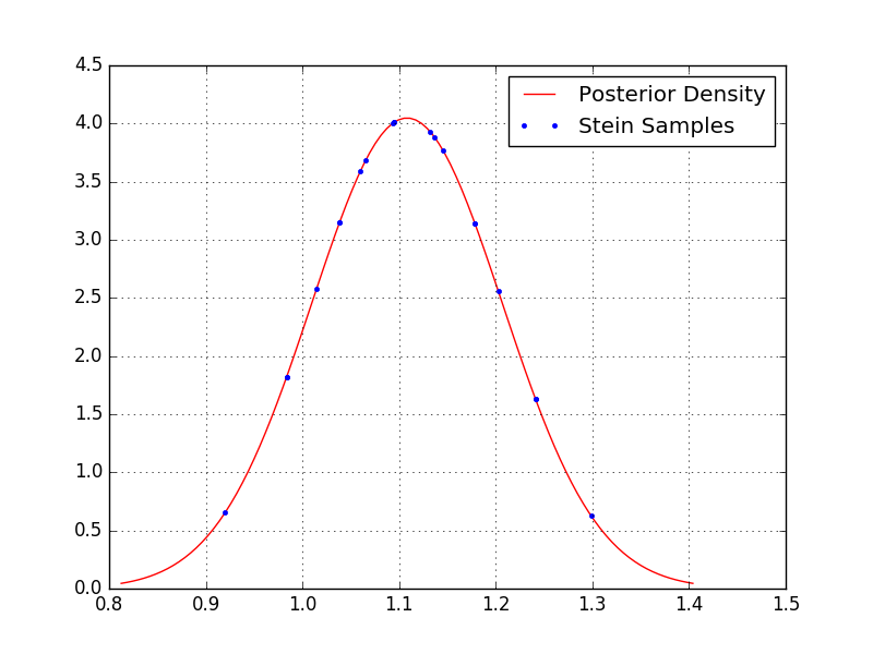By inspection we can see that more samples are concentrated about the peak of the distribution, as desired, whereas fewer samples lie out in the tails.

One might reasonably wonder how the performance changes in higher dimensions. A trivial experiment we can perform is to compare the sample mean and covariance matrix with the known posterior mean and covariance. By changing the number of linear coefficients to four and using fifty particles instead of twenty (i.e. setting k = 4 and n_particles = 50 in the code above), I can produce the following:

Posterior mean: [ 0.85912124  0.8707046   0.96091313  0.96955137]
Sample mean:    [ 0.85407118  0.86578229  0.95594568  0.96456312]

Posterior covariance:
[[ 0.00876535  0.0010954  -0.00164263 -0.0007628 ]
 [ 0.0010954   0.01099731 -0.00275835 -0.00052448]
 [-0.00164263 -0.00275835  0.01293988  0.00031979]
 [-0.0007628  -0.00052448  0.00031979  0.01042193]]

Sample covariance:
[[ 0.00773143  0.00099411 -0.00147471 -0.00068003]
 [ 0.00099411  0.00971538 -0.00249912 -0.00046036]
 [-0.00147471 -0.00249912  0.01147654  0.00030547]
 [-0.00068003 -0.00046036  0.00030547  0.00911099]]

Roughly speaking, the samples appear to approximate the expectation and covariance of the target distribution quite well!

Future Directions

In the next post in this series, I will be discussing applications of Stein variational gradient descent to estimating the weights and biases of Bayesian neural networks. This is an important area in order to allow us to utilize uncertainty in deep learning. Stay tuned!